Thursday, April 23, 2015

Kalai-Smorodinsky Solution to Bargaining Problems

1. Desired Properties
  • invariant to coordinate-wise affine transformation
  • symmetry-preserving
  • efficient
  • monotone

2. Problem Statement

We consider a two-person bargaining problem formulated as follows


  • $(a, S)$: to every two-person game we associated a pair $(a,S)$, where $a$ is a point in the plane and $S$ is a subset of the plane. 
  • The pair $(a,S)$ has the following intuitive interpretation: $a = (a_1, a_2)$ where $a_i$ is the level of utility that player $i$ receives if the two players do not cooperate with each other.
  • Every point $x = (x_1, x_2) \in S$ represents the level of utility for players 1 and 2 that can be reached by an outcome of the game which is feasible for the two players when they do cooperate. 

3. Assumption

  • Assumption 1: There is at least one point $x \in S$ such that $x^i > a_i, for i = 1,2$. In other words, bargaining may prove worthwhile for both players.
  • Assumption 2: $S$ is convex. This is justified under the assumption if two outcomes of the game give raise to points $x$ and $y$ in $S$, then randomization of these two outcomes give raise to all convex combinations of $x$ and $y$. 
  • Assumption 3: $S$ is compact. 
  • Assumption 4: $a \leq x$ for every $x \in S$. If this is not the case, we can disregard all the points of $S$ that fail to satisfy this condition because it is impossible that both players will agree to such a solution.

4. Axioms
We let $U$ denote the set of pairs $(a,S)$ that satisfying these four conditions, and we call an element in $U$ a bargaining pair.


  • Axiom 1: Pareto Optimality
    • For every $(a,S) \in U$ there is no $y \in S$ such that $y \geq f(a,S)$ and $y \neq f(a,S)$. 
  • Axiom 2: Symmetry
    • We let $T: R^2 \rightarrow R^2$ be defined by $T((x_1, x_2)) = (x_2, x_1)$ and we require that for every $(a,S) \in U$, $f(T(a), T(S)) = T(f(a,s))$.
  • Axiom 3: Invariance with Respect to Affine Transformation of Utility
    • A is an afine transformation of utility if $A = (A_1, A_2): R^2 \rightarrow R^2$, $A((x_1, x_2)) = (A(x_1), A(x_2))$, and the maps $A_i(x)$ are of the form $cx_i + d_i$ for some positive constant $c_i$ and some constant $d_i$. We require that for such a transformation $A$, $f(A(a), A(S)) = A(f(a,S))$.
In addition to the above three axioms, Nash introduced the following
  • Axiom of Independence of Irrelavant Alternatives
    • If $(a,S)$ and $(a, T)$ are bargaining pairs such that $S \subset T$ and $f(a,T) \in S$, then $f(a,T) = f(a,S)$. 
    • Interpretation: given a bargaining pair $(a,S)$, for every point $x = (x_1, x_2) \in S$, consider the product $(x_1 - a_1) (x_2 - a_2)$. Then $\eta(a,S)$ is the unique point in $S$ that maximizes this product.
    • Many objectives are raised to Nash's axiom of independence of irrelevant alternatives.  
We define some notations, 
  • $b_1 (s) = sup \{x \in R; \mbox{ for some } y \in R (x,y) \in S\}$
  • $b_2 (s) = sup \{y \in R; \mbox { for some } x \in R (x,y) \in S\}$
  • Let $g_s(x)$ be a function defined for $x \leq b_1(s)$ in the following way
    • $g_s(x) = y$ if $(x,y)$ is the Pareto of $(a,s)$. 
    • $g_s(x) = b_s(S)$ if there is no such $y$.
    • thus $g_s(x)$ is the maximum player 2 can get if player 1 get at least x. 
  • By assumption 1 in the definition of a bargaining pair $b_i(S) > a_i$. 
  • By the compactness of $S$, $b_1(S)$ and $b_2(S)$ are finite and are attained by points in $S$. 
  • A pair $(a,S)$ will be called normalized if $a = 0 = (0,0)$ and $b(S) = (1,1)$. Clearly every game can be normalized by a unique affine transformation of the utilities. 
Example objective to Nash's Solution: consider the following two normalized pair $(0,S_1)$ and $(0,S_2)$ where


  • $S_1$ = convex hull, ${(0,1), (1,0), (0.75, 0.75)}$ and 
  • $S_2$ = convex hull, ${(0,1), (1,0), (1, 0.7)}$
  • Nash's solution for $(0,S_1)$ is $(0.75, 0.75)$, and $(1, 0.7)$ for $(0,S_2)$. 
  • Limitations pf Nash's solution: Player 2 has good reasons to demand that he get more in the bargaining pair $(0,S_2)$ than he does in $(0,S_1)$. 
In order to overcome this limitation, Kalai suggests the following alternative axiom.

Axiom of Monotonicity: If $(a,S_2)$ and $(a, S_1)$ are bargaining pairs such that $b_1(S_1) = b_1(S_2)$ and $g_{s_1} = g_{s_2}$, then $f_2(a,S_1) = f_2(a,S_2)$ (where $f(a,S) = (f_1(a,S), f_2(a,S))$. 

  • This axiom states that if, for every utility level that player 1 may demand, the maximum feasible utility level that player 2 can simultaneously reach is increased, then the utility level assigned to player 2 according to the solution should also be increased. 
Theorem: There is one and only one solution, $\mu$, satisfying the axioms of monotonicity. The function $\mu$ has the following simple representation. For a pair $(a,S) \in U$ consider the line joining a to be $b(S)$, $L(a,b(S))$. The maximal element (with partial order of $R^2$) of $S$ on this line is $\mu(a,S)$. 


5. How does it work
  • to normalize the utility function of each agent in such a way that it is worth zero at the status quo and one at this agent's best outcome -- given that all others get at least their status quo utility level
  • to sharing equally the benefits of cooperation. In other words, this solution equalizes the relative benefit from status quo or equivalently the relative frustration until the shadow optimum. 

6. Solution

  • Independence of irrelevant alternatives can be substituted with a monotonicity condition. It is the point which maintains the ratios of maximal gains. In other words, if player 1 could receive a maximum of $g_1$ with player 2's help (and vice versa for $g_2$), then the bargaining solution would yield the point $\phi$ on the Pareto frontier such that $\phi_1 / \phi_2 = g_1/ g_2$.


References

[1] Bargaining problem, wiki
[2] Other solutions to Nash's bargaining problem, by Ehud Kalai, Meir Smorodinsky, in STOR 1975

Summary of Nash Bargaining


1. Bargaining problems Scenarios
Bargaining problems represent situations in which
  • There is a conflict of interest about agreements.
  • Individual have the possibility of concluding a mutually beneficial agreements.
  • No agreement may be imposed on any individual without his approval

2. Bargaining problem Definition
Example: Suppose 2 players must split one unit of good. If no agreement is reached, then players do not receive anything. We define the following notations.
  • $X$: the set of possible agreements
    • X = {$x_1$, $x_2$)| $x_1 + x_2 = 1$, $x_i \geq 0$}
  • $D$: the disagreement outcome
    • D = (0,0)
  • $u_i$: each player i has preferences, represented by a utility function $u_i$ over $X \cup {D}$
Definition: a bargaining problem is then defined as a pair of $(U,d)$ where $U \in R^2$ and $d \in U$. We assume that
  • $U$ is a convex and compact set
  • There exists some $v \in U$ such that $v > d$ (i.e., $v_i > d_i$ for some i)

3. Axioms
  • Pareto Efficiency
    • A bargaining solution $f(U,d)$ is Pareto efficient if there does not exist a $(v_1, v_2) \in U$ such that $v \geq f(U,d)$ and $v_i > f_i(U,d)$ for some $i$. 
    • An inefficient outcome is unlikely, since it leaves space for renegotiation.
  • Symmetry
    • Let $(U,d)$ be such that $(v_1, v_2) \in U$ if and only if $(v_2, v_1) \in U$ and $d_1 = d_2$. Then $f_1(U,d) = f_2 (U,d)$.
    • If the players are indistinguishable, the agreement should not discriminate between them.
  • Invariance to Equivalent Payoff Representations
    • Given a bargaining problem $(U,d)$, consider a different bargaining problem $(U', d')$, for some $\alpha >0, \beta$.
      • $U' = \{(\alpha_1 v_1 + \beta_1, \alpha_2 v_2 + \beta_2)| (v_1, v_2 \in U\}$
      • $d' = (\alpha_1 d_1 + \beta_1, \alpha_2 d_2 + \beta_2)$
    • Then $f_i(U', d') = \alpha_i f_i (U,d) + \beta_i$
    • Utility functions are only representation of preferences over outcomes. A transformation of the utility function that maintaining the same ordering over preferences (such as linear transformation) should not alter the outcome of bargaining process.
  • Independence of Irrelevant Alternatives
    • Let $(U,d)$ and $(U', d)$ be two bargaining problems such that $U' \subset U$, if $f(U,d) \in U'$, then $f(U', d) = f(U,d)$.


4. Nash Bargaining Solution
Definition: We say  that a pair of payoffs $(v^*_1, v^*_2)$ is a Nash bargaining solution if it solves the following optimization problem
  • $\max_{v_1, v_2} (v_1 - d_1)(v_2-d_2)$
  • subject to 
    • $(v_1, v_2) \in U$
    • $(v_1, v_2) \geq (d_1, d_2)$
We use $f^N(U,d)$ to denote the Nash Bargaining Solution

Remarks: 
  • Existence of an optimal solution: since the set $U$ is compact and the objective function of the problem is continuous, there exists an optimal solution for the problem
  • Uniqueness of the optimal solution: the objective function of the problem is strictly quasi-concave. Therefore, the problem has a unique solution.
Proposition: Nash bargaining solution $f^N(U,d)$ is the unique bargaining solution that satisfies the 4 axioms.


Reference
[1] Game Theory with Engineering Applications: Nash Bargaining Solution, by Asu Ozdaglar, MIT 2010

Monday, March 30, 2015

How to read technical papers in computer science?


From: http://www.cs.iit.edu/~winet/contact.html

How to read technical papers in computer science?
When you read articles or reports, keep the following in mind
  • What is the main contribution of the paper?
  • Is this important, why?
  • Is this a theoretical contribution to some fundamental problems in CS, or a protocol-like contribution, or both?
  • What was the main insight in getting the result?
  • What is not clear to you?
  • What did the authors not do, and you regard important?
  • What are the most important assumptions, are they limiting?
  • What are the possible applications suggested in the paper?
  • How does this relate to other things we have seen?
  • What extensions does this suggest?
  • Can you suggest some project idea based around the ideas in this paper

Tuesday, December 23, 2014

Introduction to Memory

1. Background

  • Program must be brought (from disk) to memory and placed within process for it to be run
  • Main memory and registers are only storage CPU can access directly
  • Memory unit only sees a stream of addresses + read requests
    • or address +data and write request
  • Register access in one CPU clock (or less)
  • Main memory can take many cycles (stalls)
  • Cache sit between main memory and CPU registers
  • Protection of memory required to ensure correct operation 
2. Address binding
  • Addresses represented in different ways at different stages of a program's life
    • source code addresses usually symbolic
    • compile code addresses bind to relocated addresses
      • i.e., 14 bytes from beginning of this module
    • Linker or loader will bind relocatable addresses to absolute addresses
    • Each binding maps one address space to another
  • Address binding of instructions and data to memory addresses can happen at three different stages
    • compile time: if memory location known a priori, absolute code can be generated; must recompile code if starting location changes
    • load time: must generate relocatable code if memory location is not known at compile time
    • execution time: binding delayed until run time if the process can be moved during its execution from one memory segment to another
      • need hardware support for address maps (e..g, base and limit registers)
3. Multistep Processing of a user program


4. Logical v.s. Physical Address Space
  • The concept of a logical address space that is bound to a separate physical address space is central to proper memory management
    • logical address: generated by the CPU; also referred to as virtual address
    • physical address: address seen by the memory unit
  • Logical and physical addresses are the same in compile-time and load-time address-binding schemes; logical (virtual) and physical addresses differ in execution-time address-binding scheme.
  • Logical address space is the set of all logical addresses generated by a program
  • Physical address space is the set of all physical addresses generated by a program
5. Dynamic loading
  • routine is not loaded until it is called
  • better memory-space utilization; unused routine is never loaded
  • all routines kept on disk is relocatable load format
  • useful when large amounts of code are needed to handle infrequently occurring cases
  • no special support from the operation system is required
    • implemented through program design
    • OS can help by providing libraries to implement dynamic loading
6. Dynamic Linking
  • Static linking
    • system libraries and program code combined by the loader into the binary program image
  • Dynamic liking
    • linking postponed until execution time
      • small piece of code, stub, used to locate the appropriate memory-resident library rountine
  • Stub replaces itself with the address of the routine, and executes the routine
  • Operating system checks if routine is in processes' memory address
    • if not in address space, add to address space
  • Dynamic linking is particularly useful for libraries
    • system also known as shared libraries
  • Consider applicability to patching system libraries
    • versioning may be needed
7. Base and Limit Registers
  • A pair of base and limit registers define the logical address space


8. Hardware address protection with base and limit registers


9. Memory Management Unit (MMU)
  • Hardware device that at run time maps virtual to physical address
  • The user program deals with logical address; it never sees the real physical addresses
    • execution-time binding occurs when reference is made to location in memory
    • logical address bound to physical address


10. Dynamic relocation using a relocation register


Job Scheduling

1. Objective

  • maximum CPU utilization obtained with multiprogramming
  • CPU-I/O Burst Cycle- Process execution consist of a cycle of CPU execution and I/O wait
2. CPU Scheduler
  • Selects from among the processes in ready queue, and allocates the CPU to one of them
    • queues may be ordered in various ways
  • CPU scheduling decisions may take place when a process
    • switches from running to waiting sate
    • switches from running to ready state
    • switches from waiting to ready state
    • terminate
  • scheduling under 1 and 4 is non-preemptive
  • all other scheduling is preemptive
    • consider access to shared data
    • consider preemption while in kernel mode
    • consider interrupts occurring during crucial OS activicites
3. Dispatcher
  • Dispacher module gives control of the CPU to the process selected by the short-term scheduler; this involves
    • switching context
    • switching to user mode
    • jumping to the proper location in the user program to restart that program
  • Dispatch latency
    • time it takes for the dispatcher to stop one process and start another running
4. Scheduling Criteria
  • CPU utilization
    • keep the CPU as busy as possible
  • Throughput 
    • # of processes that complete their execution per time unit
  • Turnaround time
    • amount of time to execute a particular process
  • Waiting time
    • amount of time a process has been waiting in the ready queue


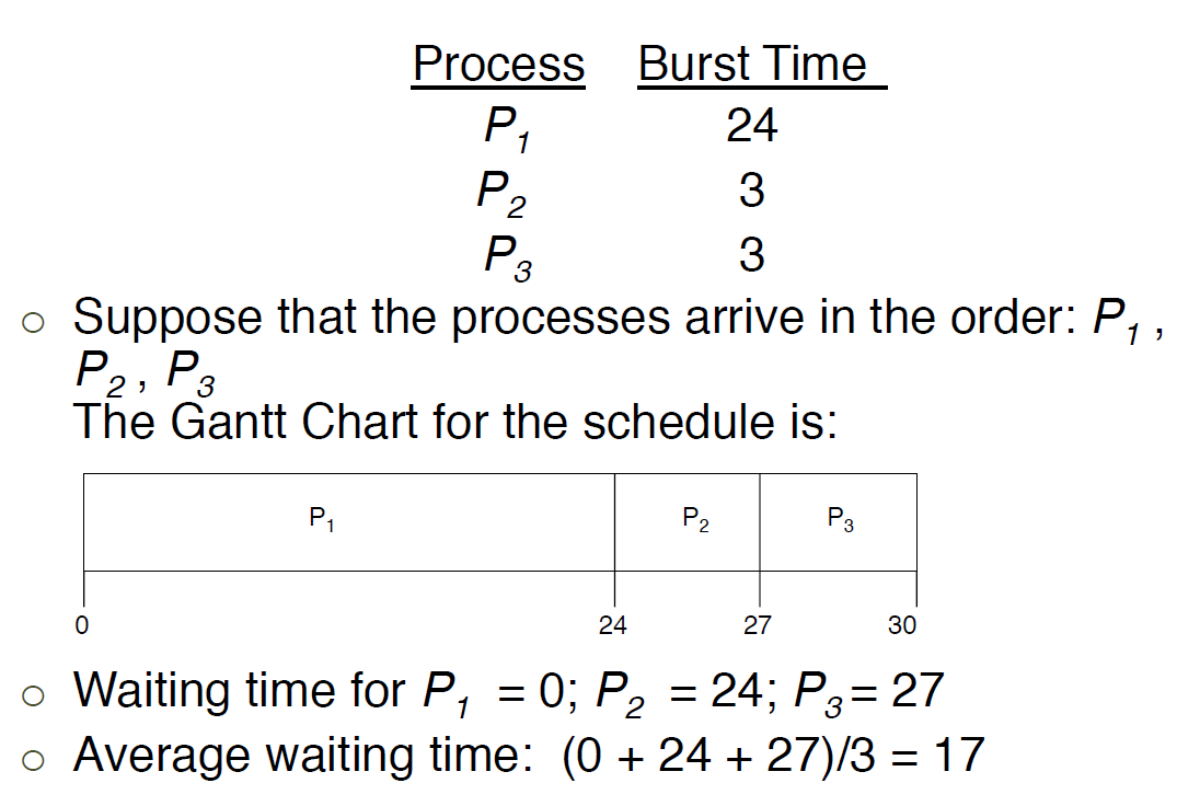
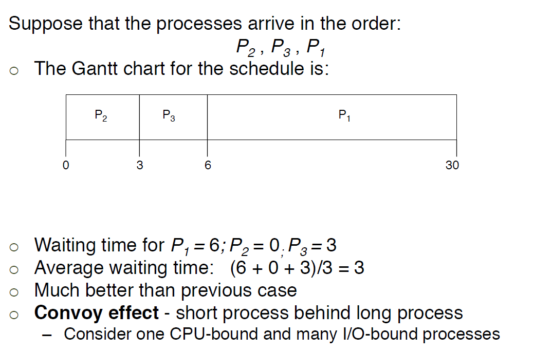
5. First-Come. First-Server (FCFS) Scheduling


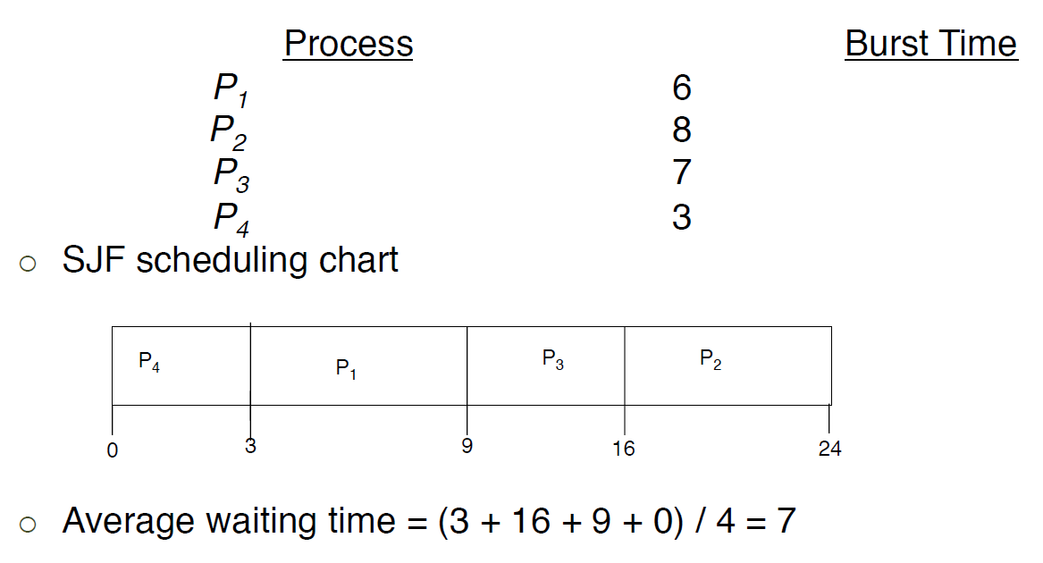
6. Shortest-Job-First (SJF) Scheduling
  • associate with each process the length of its next CPU burst
    • use these lengths to schedule the process with the shortest time
  • SJF is optimal
    • gives minimum average waiting time for a given set of processes
      • the difficult is knowing the length of the next CPU request


7. Determine the length of next CPU burst
  • can only estimate the length
    • should be similar to the previous one
    • then pick process with shortest predicted next CPU burst
  • can be done by using the length of previous CPU bursts, using exponential averaging
    • $t_n$ = average length of the n-th CPU burst
    • $\tau_{n+1}$ = predicted value of the next CPU burst
    • $\alpha, 0 \leq \alpha \leq (1-\alpha) \tau_n$
  • commonly, $\alpha$ set to 1/2
  • preemptive version called shortest-remaining-time-first
8. Example of Exponential Averaging
  • $\alpha = 0$
    • \tau_{n+1} = \tau_n
    • recent history does not count
  • $\alpha = 1$
    • $\tau_{n+1} = n \tau_n$
    • only the actual last CPU burst counts
  • If we expand the formula, we get
    • $\tau_{n+1} = \alpha \tau_n + (1-\alpha) \tau_{n-1} + ...$
    •                     $= (1-\alpha)^j \alpha \tau_{n-j} + ... $
    •                     $= (1-\alpha)^{n+1} \tau_0$
  • since both $\alpha$ and $1-\alpha$ are less than or equal to 1, each successive term has less weight than its predecessor
9. Example of Shortest Remaining-time-first


10. Priority Scheduling
  • A priority number (integer) is associated with each process
  • The CPU is allocated to the process with the highest priority (smaller integer = highest priority)
    • preemptive
    • non-preemptive
  • SJF is priority scheduling where priority is the inverse of predicted next CPU burst time
  • Problem = starvation 
    • low priority processes may never execute
  • Solution = aging
    • as time progresses, increase the priority of the process


11. Round Robin
  • Each process gets a small unit of CPU time (time quantum q), usually 10-100 milliseconds.
    • after this time has elapsed, the process is preempted and added to the end of the ready queue
  • If there are n processes in the ready queue and the time quantum is q, then each process gets 1/n of the CPU time is chunks of at most q time units at once. 
    • No process waits more than (n-1)q time units.
  • Time interrupts every quantum to schedule next process
  • Performance
    • q large : FIFO
    • q small: q must be large with respect to context switch, otherwise, overhead is too high
  • Example of Round robin with time Quantum =4 


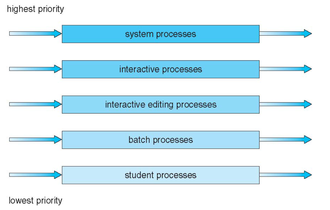
12. Multilevel Queue
  • Ready queue is partitioned into separate queues, e..g,
    • forground (iterative)
    • background (batch)
  • Process permanently in a given queue
  • Each queue has its own scheduling algorithm
    • forground-RR
    • background-FCFR
  • Scheduling must be done between the queues
    • fixed priority scheduling: i.e., serve all from foreground then from background
      • possibility starvation
    • time slices: each queue gets a certain amount of CPU time which it can schedule amongst its processes, i.e., 80% to foreground in RR
    • 20% to background in FCFS


13. Multi-level feedback queue
  • a process can move between the various queues;
  • aging can be implemented this way
  • multi-level-feedback-queue scheduler defined by the following parameters
    • number of queues
    • scheduling algorithms for each queue
    • method used to determine when to upgrade a process
    • method used to determine when to demote a process
    • method used to determine which queue a process will enter when that process needs service
  • Example of multilevel feedback queue
    • three queues
      • $Q_0$: time quantum 8 milliseconds
      • $Q_1$: time quantum 16 milliseconds
      • $Q_2$; FCFS
    • scheduling
      • a new job enters queue $Q_0$ which is served FCFS
        • when it gains CPU, job received 8 milliseconds
        • if it does not finish in 8 milliseconds, job is moved to queue $Q_1$
    • at $Q_1$ job is again served FCFS and receives 16 additional milliseconds
      • if it still does not complete, it is preempted and moved to queue $Q_2$

14. Thread Scheduling
  • Distinction between user-level and kernel-level threads
  • when threads supported, threads scheduled, not processes
  • many-to-one and many-to-many methods, thread library schedules user-level threads to run on LWP
    • known as process-contention scope (PCS) since scheduling competition is within the process
    • typically thread scheduled onto available CPU is system contention scope (SCS)
      • competition among all threads in the system
15. Multi-Processor Scheduling
  • CPU scheduling more complex when multiple CPUs are available
  • Homogeneous processors within a multiprocessor
  • Asymetric multiprocessing
    • only one processor accesses the system data structures, alleviating the need for data sharing
  • Symmetric multiprocessing (SMP)
    • each processor is self-scheduling, all processes in common ready queue
    • or each has its own private queue of ready processes
  • Processor Affinity
    • process has affinity for processor on which it is currently running
      • soft affinity
      • hard affinity
      • variation including processor sets
16. Multiplecore Processor
  • recent trend to place multiple processor cores on the same physical chip
  • faster and consumes lees power 
  • multiple threads per core also growing
    • takes advantage of memory stall to make progress on another thread while memory retrieve happens


Monday, December 22, 2014

Monitor

1. Monitor

  • high-level synchronization construct that allows the safe-sharing of an abstract data type among concurrent processes
monitor monitor-name{
    shared variable declarations
    procedure body p1(){}
    procedure body p2() {}
    procedure body pn() {}
    {
        initialization code
    }

}

2. Schematic View of a Monitor

  • the monitor construct ensures that at most one process can be active within the monitor at a given time
  • shred data (local variables) of the monitor can be accessed only by local procedure


3. Monitors Introduction

  • to allow a process to wait within the monitor
    • a condition variable must be declared, as condition x, y
  • condition variable can only be used with the operation wait and signal
    • the operation 
      • x.wait() means that the process invoking this operation is suspended until another process invokes x..signal()
      • x.signal() operation resumes exactly one suspend process on condition variable x. If no process is suspended on condition variable x, then the signal operation has no effect.
      • wait and signal operations of the monitors are not the same as semaphore wait and signal operations
4. Monitor with condition variables
  • when a process P signal to wake up process Q that was waiting on a condition, potentially both of them can be active.
  • however, monitor rules require that at most one process can be active within the monitor
    • signal and wait: P waits until Q leaves the monitor
    • signal and continue: Q waits until P leaves the monitor (or, until P waits for another condition)
    • Signal and leave: P has to leave the monitor after signaling
  • the design decision is different for different programming languages
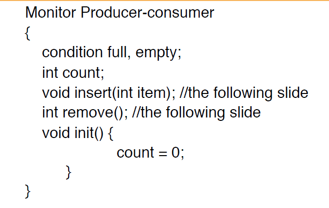
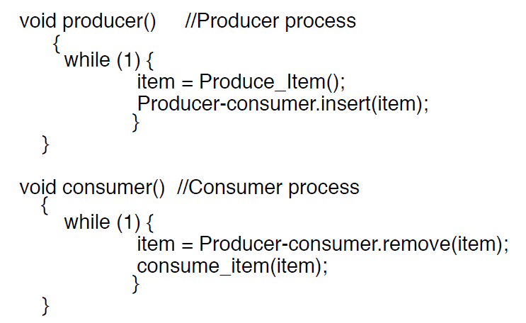
5. Procedure-Consumer Problem With Monitor


6. Dining-Phisolophers Problem with Monitors


Process Synchronization

1. Concurrent access to shared data

  • Example
    • suppose that two processes A and B have access to a shared variable "Balance"
      • process A: Balance = Balance - 100
      • process B: Balance = Balance - 200
    • Further, assume that Process A and Process B are executing concurrently in a time-shared, multiprogrammed system
    • The statement "balance = balance - 100" is implemented by several machine level instructions such as
      • A1. LOAD R1, BALANCE //load BALANCE from memory to register 1 (R1)
      • A2. SUB R1, 100 //subtract 100 from R1
      • A2. STORE BALANCE, R1 //store R1's contents back to the memory location of BALANCE
    • Similarly, "BALANCE = BALANCE - 200" can be implemented in the following
      • B1. LOAD R1, BALANCE
      • B2. SUB R1, 200
      • B3. STORE BALANCE, R1
2. Race Condition
  • Observe: in a time-shared system, the exact instruction execution order cannot be predicted
  • Situations like this, where multiple processes are writing or reading some shared data and the final result depends on who runs precisely when, are called race conditions.
  • A serious problem for any concurrent system using shared variables.
  • We must make sure that some high-level code sections are executed atomically.
  • Atomic operation means that it completes in its entirety without worrying about interruption by an other potentially conflict-causing process.
3. The Critical-Section Problem
  • n processes are competing to use some shared data
  • Each process has a code segment, called critical section (critical region), in which the shared data is accessed.
  • Problem: ensure that when one process is executing in its critical section, no other process is allowed to execute in that critical section.
  • The execution of the critical sections by the processes must be mutually exclusive in time
4. Solving Critical-Section Problem
Any solution to the problem must satisfy four conditions
  • Mutual Exclusion
    • no two processes may be simultaneously inside the same critical section
  • Bounded Waiting
    • no process should have to wait forever to enter a critical section
  • Progress
    • no process executing a code segment unrelated to a given critical section can block  another process trying to enter the same crtical section
  • Arbitrary speed
    • no assumption can be made about the relative speed of different processes (though all processes have a non-zero speed)
5. General Structure of a Typical Process

do{
...
entry section
     critical section
exit section
     remainder section
} while(1);

  • we assume this structure when evaluating possible solutions to Critical Section Problem
  • in the entry section, the process requests "permission"
  • we consider single-processor systems

5. Getting help from hardware
  • one solution supported by hardware may be to use interrupt capability
do{
     DISABLE INTERRUPTS
          critical section;
     ENABLE INTERRUPTS
         remainder section

} while(1);


6. Synchronization Hardware
  • Many machines provide special hardware instructions that help to achieve mutual exclusion
  • The TestAndSet (TAS) instruction tests and modifies the content of a memory word automatically
  • TAS R1, LOCK
    • reads the contents of the memory workd LOCK into register R!
    • and stores a nonzero value (e.g. 1) at the memory word LOCK (again, automatically)
      • assume LOCK = 0;
      • calling TAS R1, LOCK will set R! to 0, and set LOCK to 1
      • Assume lOCK = 1
      • calling TAS R1 LOCK will set R1 to 1, and set LOCK to 1
7. Mutual Exclusion with Test-and-Set
  • Initially, share memory word LOCK = 0;
  • Process pi
do{
     entry-section:
      TAS R1, LOCK
      CMP R1, #0
      JNE entry_section //if not equal, jump to entry
         critical section
      MOVE LOCK, #0 //exit section
         remainder section
} while(1);


8. Busy waiting and spin locks
  • This approach is based on busy waiting: if the critical section is being used, waiting processes loop continuously at the entry point
  • a binary lock variable that uses busy waiting is called "spin lock"
9. Semaphores
  • Introduced by E.W. Dijkstra
  • Motivation: avoid busy waiting by locking a process execution until some condition is satisfied
  • Two operations are defined on a semaphore variable s
    • wait(s): also called P(s) or down(s)
    • signal(s): also called V(s) or up(s)
  • We will assume that these are the only user-visible operations on a semaphore 
10. Semaphore Operations
  • Concurrently a semaphore has an integer value. This value is greater than or equal to 0
  • wait(s)
    • wait/block until s.value > 0 //executed atomatically
  • a process executing the wait operation on a semaphore, with value 0 is blocked until the semaphore's value become greater than 0
    • no busy waiting
  • signal(s)
    • s.value++ //execute automatically
  • If multiple processes are blocked on the same semaphore "s", only one of them will be awakened when another process performs signal(s) operation
  • Semaphore as a general synchronization tool: semaphores provide a general process synchronization mechanism beyond the "critical section" problem

11. Deadlocks and Starvation
  • A set of processes are aid to be in a deadlock state when every process in the set is waiting for an even that can be caused by another process in the set
  • A process that is forced to wait indefinitely in a  synchronization program is said to be subject to starvation
    • in some execution scenarios, that process does not make any progress
    • deadlocks imply starvation, bu the reverse is not true
12. Classical problem of synchornization
  • Produce-Consumer Program
  • Readers-Writer Problem
  • Dining-Philosophers Problem
  • The solution will use only semaphores as synchronization tools and busy waiting is to be avoided.
13. Producer-Consumer Problem
  • Problem
    • The bounded-buffer producer-consumer problem assumes there is a buffer of size n
    • The producer process puts items to the buffer area
    • The consumer process consumes items from the buffer
    • The producer and the consumer execute concurrently
  • Make sure that
    • the producer and the consumer do not access the buffer area and related variables at the same time
    • no item is made available to the consumer if all the buffer slots are empty
    • no slots in the buffer is made available to the producer if all the buffer slots are full
  • Shared data
    • semaphore full, empty, mutex
  • Initially
    • full = 0; //the number of full buffers
    • empty = n; //the number of empty buffers
    • mutex = 1; // semaphore controlling the access to the buffer pool
  • Producer Process

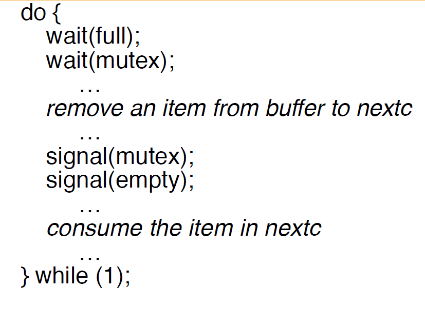
  • Consumer Process


14. Readers-Writers Problem

  • Problem
    • A data object( e.g. a file) is to be shared among several concurrent processes
    • A write process must have exclusive access to the data object
    • Multiple reader processes may access the shared data simultaneously without a problem
  • Shared data
    • semaphore mutex, wrt
    • int readaccount
  • Initially
    • mutex = 1
    • readcount = 0, wrt= 1
  • Writer Process

  • Read Process

15. Dining-Philosophers Problem
  • Problem
    • five phisolophers share a common circular table
    • there are five chopsticks and a bowl of rice (in the middle)
    • when a philosopher gets hungry, he tries to pick up the closest chopsticks
    • a philosopher may pick up only one chopstick at a time, and he cannot pick up one that is already in use. 
    • when done, he puts down both of his chopsticks, one after the other.
  • Shared Data
    • semaphore chopsticks [5]
  • Initially
    • all semaphore values are 1