Job Scheduling

1. Objective

• maximum CPU utilization obtained with multiprogramming
• CPU-I/O Burst Cycle- Process execution consist of a cycle of CPU execution and I/O wait

2. CPU Scheduler

• Selects from among the processes in ready queue, and allocates the CPU to one of them
• queues may be ordered in various ways
• CPU scheduling decisions may take place when a process
• switches from running to waiting sate
• switches from running to ready state
• switches from waiting to ready state
• terminate
• scheduling under 1 and 4 is non-preemptive
• all other scheduling is preemptive
• consider access to shared data
• consider preemption while in kernel mode
• consider interrupts occurring during crucial OS activicites

3. Dispatcher

• Dispacher module gives control of the CPU to the process selected by the short-term scheduler; this involves
• switching context
• switching to user mode
• jumping to the proper location in the user program to restart that program
• Dispatch latency
• time it takes for the dispatcher to stop one process and start another running

4. Scheduling Criteria

• CPU utilization
• keep the CPU as busy as possible
• Throughput 
• # of processes that complete their execution per time unit
• Turnaround time
• amount of time to execute a particular process
• Waiting time
• amount of time a process has been waiting in the ready queue

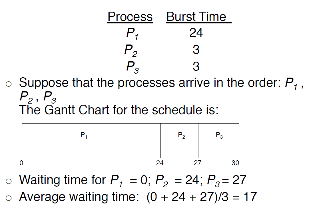
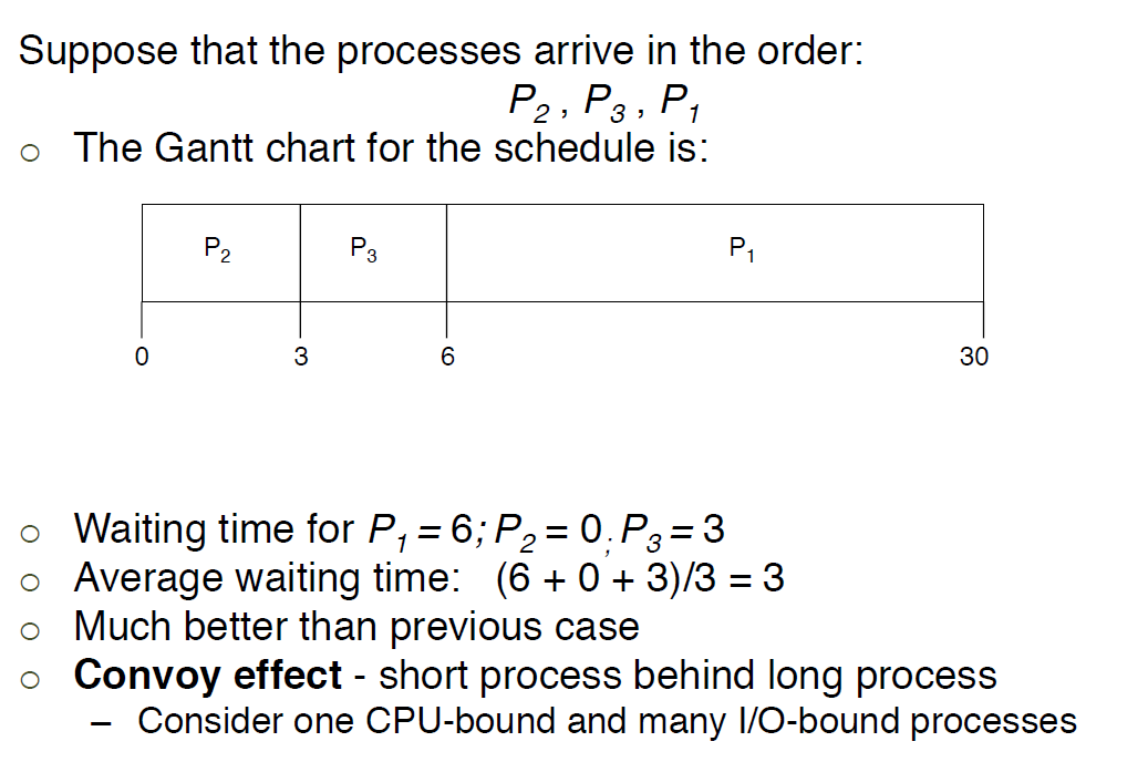
5. First-Come. First-Server (FCFS) Scheduling

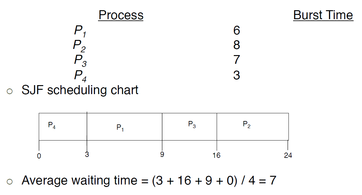
6. Shortest-Job-First (SJF) Scheduling

• associate with each process the length of its next CPU burst
• use these lengths to schedule the process with the shortest time
• SJF is optimal
• gives minimum average waiting time for a given set of processes
• the difficult is knowing the length of the next CPU request

7. Determine the length of next CPU burst

• can only estimate the length
• should be similar to the previous one
• then pick process with shortest predicted next CPU burst
• can be done by using the length of previous CPU bursts, using exponential averaging
• $t_n$ = average length of the n-th CPU burst
• $\tau_{n+1}$ = predicted value of the next CPU burst
• $\alpha, 0 \leq \alpha \leq (1-\alpha) \tau_n$
• commonly, $\alpha$ set to 1/2
• preemptive version called shortest-remaining-time-first

8. Example of Exponential Averaging

• $\alpha = 0$
• \tau_{n+1} = \tau_n
• recent history does not count
• $\alpha = 1$
• $\tau_{n+1} = n \tau_n$
• only the actual last CPU burst counts
• If we expand the formula, we get
• $\tau_{n+1} = \alpha \tau_n + (1-\alpha) \tau_{n-1} + ...$
•                     $= (1-\alpha)^j \alpha \tau_{n-j} + ... $
•                     $= (1-\alpha)^{n+1} \tau_0$
• since both $\alpha$ and $1-\alpha$ are less than or equal to 1, each successive term has less weight than its predecessor

9. Example of Shortest Remaining-time-first

10. Priority Scheduling

• A priority number (integer) is associated with each process
• The CPU is allocated to the process with the highest priority (smaller integer = highest priority)
• preemptive
• non-preemptive
• SJF is priority scheduling where priority is the inverse of predicted next CPU burst time
• Problem = starvation 
• low priority processes may never execute
• Solution = aging
• as time progresses, increase the priority of the process

11. Round Robin

• Each process gets a small unit of CPU time (time quantum q), usually 10-100 milliseconds.
• after this time has elapsed, the process is preempted and added to the end of the ready queue
• If there are n processes in the ready queue and the time quantum is q, then each process gets 1/n of the CPU time is chunks of at most q time units at once. 
• No process waits more than (n-1)q time units.
• Time interrupts every quantum to schedule next process
• Performance
• q large : FIFO
• q small: q must be large with respect to context switch, otherwise, overhead is too high
• Example of Round robin with time Quantum =4 

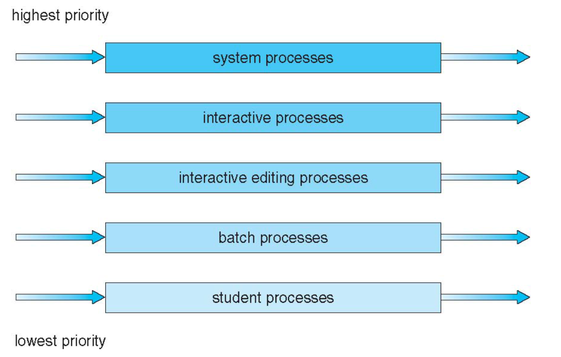
12. Multilevel Queue

• Ready queue is partitioned into separate queues, e..g,
• forground (iterative)
• background (batch)
• Process permanently in a given queue
• Each queue has its own scheduling algorithm
• forground-RR
• background-FCFR
• Scheduling must be done between the queues
• fixed priority scheduling: i.e., serve all from foreground then from background
• possibility starvation
• time slices: each queue gets a certain amount of CPU time which it can schedule amongst its processes, i.e., 80% to foreground in RR
• 20% to background in FCFS

13. Multi-level feedback queue

• a process can move between the various queues;
• aging can be implemented this way
• multi-level-feedback-queue scheduler defined by the following parameters
• number of queues
• scheduling algorithms for each queue
• method used to determine when to upgrade a process
• method used to determine when to demote a process
• method used to determine which queue a process will enter when that process needs service
• Example of multilevel feedback queue
• three queues
• $Q_0$: time quantum 8 milliseconds
• $Q_1$: time quantum 16 milliseconds
• $Q_2$; FCFS
• scheduling
• a new job enters queue $Q_0$ which is served FCFS
• when it gains CPU, job received 8 milliseconds
• if it does not finish in 8 milliseconds, job is moved to queue $Q_1$
• at $Q_1$ job is again served FCFS and receives 16 additional milliseconds
• if it still does not complete, it is preempted and moved to queue $Q_2$

14. Thread Scheduling

• Distinction between user-level and kernel-level threads
• when threads supported, threads scheduled, not processes
• many-to-one and many-to-many methods, thread library schedules user-level threads to run on LWP
• known as process-contention scope (PCS) since scheduling competition is within the process
• typically thread scheduled onto available CPU is system contention scope (SCS)
• competition among all threads in the system

15. Multi-Processor Scheduling

• CPU scheduling more complex when multiple CPUs are available
• Homogeneous processors within a multiprocessor
• Asymetric multiprocessing
• only one processor accesses the system data structures, alleviating the need for data sharing
• Symmetric multiprocessing (SMP)
• each processor is self-scheduling, all processes in common ready queue
• or each has its own private queue of ready processes
• Processor Affinity
• process has affinity for processor on which it is currently running
• soft affinity
• hard affinity
• variation including processor sets

16. Multiplecore Processor

• recent trend to place multiple processor cores on the same physical chip
• faster and consumes lees power 
• multiple threads per core also growing
• takes advantage of memory stall to make progress on another thread while memory retrieve happens