Time Series Models (ARIMA)

Anomaly Detection

1.  Data Labels

• Supervised Anomaly Detection
• labels available for both normal data and anomalies
• similar to rare class mining
• Semi-supervised Anomaly Detection
• labels available only for normal data
• Unsupervised Anomaly Detection
• No labels assumed
• Based on the assumption that anomalies are very rare compared to normal data

2. Type of Anomalies

P

• Point Anomalies
• An individual data instance is anomalous w.r.t. the data

• Contextual Anomalies
• An individual data instance is anomalous within a context 
• requires a notion of context
• also referred to as conditional anomalies

• Collective Anomalies
• A collection of related data instances is anomalous
• Requires a relationship among data instances
• sequential data
• spatial data
• graph data
• The individual instances within a collective anomaly are not anomalous by themselves

3. Evaluation of Anomaly Detection

• Accuracy is not sufficient metric for evaluation

• Recall: $= \frac{TP}{TP+FN}$
• Precision $=\frac{TP}{TP+FP}$
• F-measure $= \frac{2*P*R}{R+P}$
• Recall (detection rate)
• ratio between the number of correctly detected anomalies and the total number of anomalies
• False alarm (false positive)
• ratio between the number of data records from normal class that are misclassified as anomalies and the total number of data records from normal class.
• ROC curve: a tradeoff between detection rate and false alarm rate.
• Area under the ROC curve (AUC) is computed using a tapeziod rule.

4. Taxonomy

5. Classification Based Techniques

• Main idea: build a classification model for normal (and anomalous (rare)) events based on labeled training data, and use it to classify each new unseen event.
• Classification models must be able to handle skewed (imbalanced) class distribution
• Categories
• supervised learning techniques
• require knowledge of both normal and anomaly class
• build classifier to distinguish between normal and known anomalies
• semi-supervised classification techniques
• require knowledge of normal class only
• use modified classification model to learn the normal behavior and then detect any deviations from normal behavior as anomalous
• Advantage
• supervised learning techniques
• models that can be easily understood
• high accuracy in detecting many kinds of known anomalies
• semi-supervised classification techniques
• models that can be easily  understood
• normal behavior can be accurately learned
• Drawbacks
• supervised learning techniques
• require both labels from both normal and anomaly class
• cannot detect unknown and emerging anomalies
• semi-supervised classification techniques
• require labels from normal class
• possible high false alarm rate
• previous unseen data records may be recognized as anomalies

6. Nearest Neighbor Based

• Key assumption
• normal points have close neighbors while anomalies are located far from other points
• Two approach
• compute neighborhood for each data record
• analyze the neighbor to determine whether data record is anomaly or not
• Categories
• distance-based methods
• anomalies are data points most distant from other points
• density-based methods
• anomalies are data points in low density regions
• Advantage
• can be used in unsupervised or semi-supervised setting (do not make any assumptions about data distribution)
• Drawbacks
• if normal points do not have sufficient number of neighbors the techniques may fail
• computationally expensive
• in high dimensional spaces, data is sparse and the concept of similarity may not be meaningful anymore
• due to the sparseness, distances between any two data records may become quite similar
• each data record may be considered as potential outlier

7. Clustering-based Techniques

• Key assumption
• normal data records belong to large and dense clusters, while anomalies do not belong to any of the clusters or form very small clusters
• Categorization according to labels
• semi-supervised
• cluster normal data to create models for normal behavior. If a new instance do not belong to any of the clusters or it is not close to any cluster, is anomaly.
• unsupervised
• post processing is needed after a clustering step to determine the size of the clusters and the distance from the cluster is required for the point to be anomaly
• Advantage
• No need to be supervised
• Easily adaptable to online/incremental mode suitable for anomaly detection from temporal data
• Drawbacks
• computationally expensive
• using indexing structures may alleviate this problem
• if normal points do not create any clusters the techniques may fail
• in high dimensional spaces, data is sparse and distances between any two data records may become quite similar

8. Statistics Based Techniques

• Data points are modeled using stochastic distribution
• points are determined to be outliers depending on their relationship with their model
• Advantage
• utilize existing statistical modeling techniques to model various type of distributions
• Drawback
• with high dimensions, difficult to estimate distributions
• parametric assumptions often do no hold for real data sets
• Parametric Techniques
• assume that the normal (and possibly anomalous) data is generated from underlying parametric distribution
• learn the parameters from the normal sample
• determine the likelihood of a test instance to be generated from this distribution to detect anomalies
• Non-parametric Techniques
• do not assume any knowledge of parameters
• use non-parametric techniques to learn a distribution 
• e.g., parzen window estimation

9. Information Theory Based Techniques

• Computer information content in data using information theoretic measures 
• e.g., entropy, relative entropy, etc.
• Key idea: outliers significantly alter the information content in a dataset
• Approach: detect data instances that significantly alter the information content
• require an information theoretic measure
• Advantage
• operate in an unsupervised mode
• Drawback
• require an information theoretic measure sensitive enough to detect irregularity induced by few outliers
• Example
• Kolmogorov complexity
• detect smallest data subset whose removal leads to maximum reduction in kolmogorov complexity
• Entropy-based approaches
• find a k-sized subset whose removal leads to the maximal decrease in entropy

10. Spectral Techniques

• Analysis based on eigen decomposition of data
• key idea
• find combination of attributes that capture bulk of variability
• reduced set of attributes can explain normal data well, but not necessarily the outliers
• Advantage
• can operate in an unsupervised mode
• Drawback
• based on the assumption that anomalies and normal instances are distinguishable in the reduced space
• Several methods use Principal Component Analysis
• top few principal components capture variability in normal data
• smallest principal component should have constant values
• outliers have variability in the smallest component

11. Collective Anomaly Detection

• Detect collective anomalies
• Exploit the relationship among data instances
• Sequential anomaly detection
• detect anomalous sequence
• Spatial anomaly detection
• detect anomalous sub-regions within a spatial data set
• Graph anomaly detection
• detect anomalous sub-graphs in graph data

Mining Contrast Sets

1. Introduction

• Motivation
• understanding differences between groups
• Task
• provide an efficient algorithm for mining contrast contrast sets and pruning rules to reduce complexity
• provide post processing techniques to present subsets that are surprising
• control the false positives
• be statistically sound
• Goal
• To find contrast-sets whose support differs meaningfully (statistically) across groups
• $\exists i,j$  $P(cset = true | G_i) \neq P(cset = true | G_j) $, $max_{ij} | sup(cset, G_i) - sup(cset, G_j)| \geq min dev$

2. Naive Approach

• Add an attribute to the set (group type) and use Association Rule Mining to find the differences
• Problems
• this will not return group differences
• the results will be difficult to interpret

Association Rule Mining

1. Definition

• Association: Given a set of transactions, find rules that will predict the occurrence of an item based on the occurrence of other items in the transaction. 
• Support count ($\sigma$): frequency of occurrence of an itemset
• Support: fraction of transactions that contain an item set
• Frequent Itemset: An itemset whose support is greater or equal to a minsup threshold

2. Association rule

• Association rule
• $ X \rightarrow Y $
• support (s)
• fraction of transactions that contains both X and Y
• confidence
• measures how often items in Y appear in transactions that contains X

3. Association Rule Mining Task

• Given a set of transactions T, the goal of association rule mining is to find all rules having 
• support >= minsup threshold
• confidence >= minconf threshold
• Brute-force approach
• list all possible association rules
• compute the support and confidence for each rule
• prune rules that fail the minsup and minconf thresholds
• this is computationally prohibitive!

4. Two-step Approach

• Step 1: frequent itemset generation
• generate all itemset whose support >= minsup
• Step 2: rule generation
• generate high confidence rules from each frequent itemset, where each rule is a binary partitioning of a frequent itemset
• Drawback: frequent itemset generation is still computationally expensive

5. Computational Complexity

• Given d unique items
• total number of item set is: $2^d$
• total number of possible association rules is:
•  $ R = \sum^{d-1}_{k=1} [\binom{d}{k} *\sum^{d-k}_{j=1}\binom{d-k}{j}]$ = $3^d - s^{d+1} +1 $

6. Reducing Number of Candidates

• Apriori principal
• If an itemset is frequent, then all of its subsets must also be frequent
• i.e., $\forall X, Y: X \subset Y \rightarrow S(X) \geq S(Y)$
• Apriori algorithm
• Let k = 1
• generate frequent itemset of length 1
• repeat until no new frequent itemsets are identified
• generate length (k+1) candidate itemsets from length k frequent itemsets
• prune candidate itemsets containing subsets of length k that are infrequent 
• count the support of each candidate by scanning the db
• eliminate candidates that are infrequent, leaving only those that are frequent

7. Closed Itermset

• An itemset is closed if none of its immediate supersets has the same support as the itemset.

8. Effect of Support Distribution

• How to set the appropriate minsup threshold?
• if minsup is set too high, we could miss items involving interesting rate items (e.g., expensive products)
• if minsup is set too low, it is computatinally expensive and the number of itemset is very large.
• Using a single minimum support threshold may not be effective.

Clustering Measurements

1. Measures the Cluster Validity

• Numerical measures that are applied to judge various aspects of cluster validity, are classified into the following three types
• External Index: Used to measure the extent to which cluster labels match externally supplied class labels
• entropy
• Internal Index: Used to measure the goodness of a clustering structure without respect to the external information
• sum of squared error (SSE)
• Relative Index: used to compare two different clustrings of clusters
• often an external or internal index is used for this function, e.g., SSE or entropy

2. Measuring Cluster Validity via Correlation

• Two matrix
• Proximity Matrix
• Incidence Matrix
• one row and one column for each data point
• an entry is 1 if the associated pair of points belong to the same cluster, else 0
• Compute the correlation between the two matrices
• since the matrices are symmetric, only the correlation between n(n-1)/2 entries needs to be calculated 
• High correlation indicates that points that belong the same cluster are closed to each other
• Not a good measure for some density 

Large Clustering Problems

1. The Canopies Approach

• Two distance metrics
• cheap & expensive
• First pass
• very inexpensive distance metric
• create overlapping canopies
• Second pass
• expensive, accurate distance metric
• canopies determine which distances calculated

2. Using Canopies

• Calculate expensive distances between points in the same canopy
• All other distances default to infinity
• Use finite distances and iteratively merge closest

3. Preserve Good Clustering

• Small, disjoint canopies
• big time savings
• Large, overlapping canopies
• original accurate clustering
• Goal: fast and accurate
• For every cluster, there exists a canopy such that all points in the cluster are in the canopy

DBScan

1. DBScan

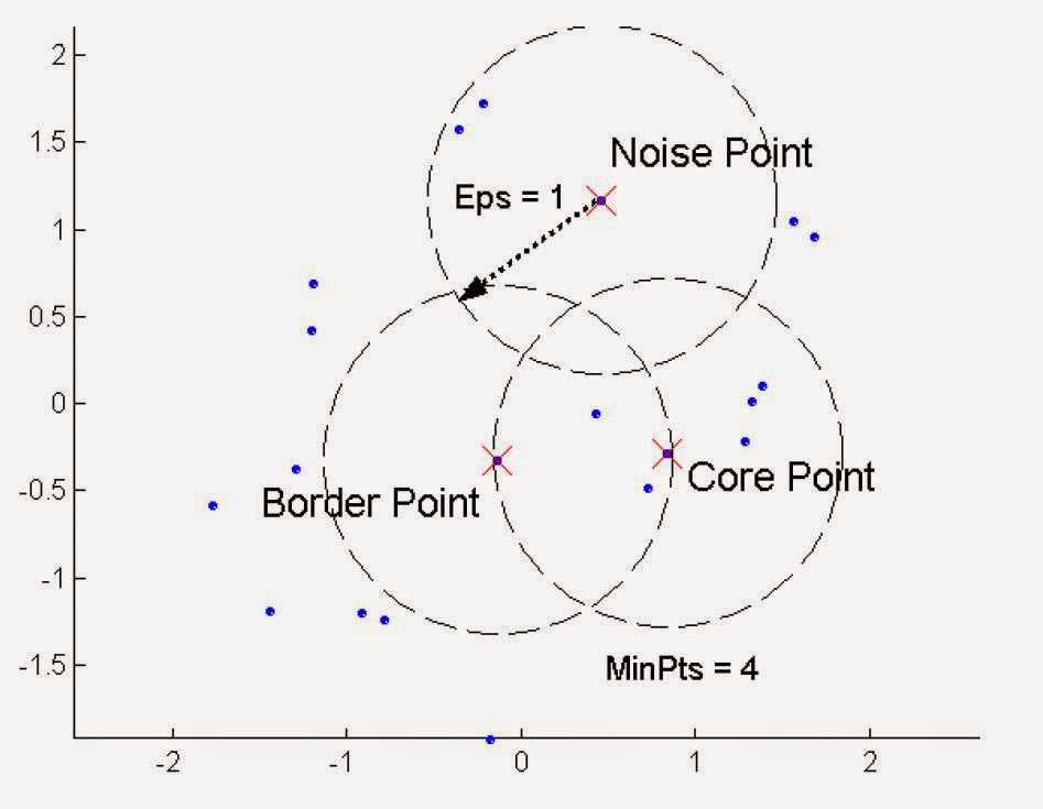
• DBScan is a density-based algorithm
• density = number of points with a specified radius (Eps)
• a point is a core point if it has more than a specified number of point (MinPts) within Eps
• There are points that are at the interior of a cluster
• A boarder point has fewer then MinPts within Eps, but is the neighborhood of a core point
• A noise point is any point that is not a core point or a boarder point.

2. DBScan Algorithm

3. Strongness v.s. Weakeness

• Strongness
• Resistant to noise
• Can handle clusters of different shapes and sizes
• Weakness
• when dataset has varying densities
• high dimensional data

4. Determine EPS and MinPts

• The idea is that for points in a cluster, their k-th nearest neighbors are at roughly the same distance
• Noise points have the kth nearest neighbor at farther distance

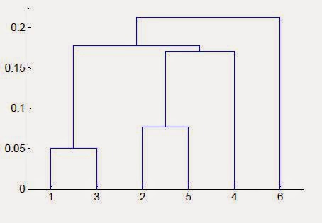
Hierarchical Clustering

1. Hierarchical Clustering

• Produces a set of nested clusters
• organized as a hierarchical tree
• Can be visualized as a dendrogram
• a tree like diagram that records the split
  

2. Strengths of Hierarchical Clustering

• Do not have to assume any particular number of clusters
• any desired number of clusters can be obtained by "cutting" the dendogram at the proper level
• They may correspond to meaning taxonomies
• example in biological sciences (e.g., animal kingdom, phylogeny reconstruction, ...)

3. Two main types of Hierarchical Clustering

• Agglomerative
• Start with the points as individual clusters
• At each step, merge the closest pair of clusters until only one cluster (or k clusters) left. 

• Divisive
• Start with one, all-inclusive cluster
• At each step, split a cluster until each cluster contains a point (or there are k clusters)

4. Inter-Cluster Similarity

• Min
• strength: can handle non-elliptical shapes
• weakness: sensitive to noise and outliers
• Max
• strength: less susceptible to noise and outliers
• weakness: tend to break large clusters; biased towards globular clusters
• Group Average
• proximity of two clusters is the average of pairwise similarity between points in the two clsuters

$Proximity = \frac{\sum_{p_i \in Cluster_i, P_j \in cluster_j}{Proximity(p_i, p_j)}}{|Cluster_i||Cluster_j|}$

• Strongness: less susceptible to noise and outliers
• Weakness: biased towards globular clusters
• Distance between centroids
• Other methods driven by an objective function
• Ward's method users squared error
• Similarity of two clusters is based on the increase in squared error when two clusters are merged
• Similar to gorup average if distance between points is distance squared.
• Strongness: less susceptible to noise and outliers
• Weakness: 
• Biased towards globular clusters
• Hierarchical analogue of K-means

5. Hierarchical Clustering: Problems and Limitations

• Once a decision is made to combine two clusters, it cannot be undone
• No objective function is directly minimized
• Different schemes have problems with one or more of the following
• sensitivity to noise and outliers
• difficulty handling different sized clusters and convex shapes
• breaking large clusters

6. MST: Divisive Hierarchical Clustering

• Build MST (Minimum Spanning Tree)
• start with a tree that consists of any point
• in successive steps, look for the closest pair of points (p,q) such that one point (p) is in the current tree but the other (q) is not

Partitional Clustering

1. Partitional Clustering v.s. Hierarchical Clustering

• Partitioning clustering: A division of data objects into non-overlapping subsets (clusters) such that each data object is in exactly one subset.
• Hierarchical clustering: A set of nested clusters organized as a hierarchical tree.

2. Types of Cluster

• Well-Separated Clusters: a cluster is a set of points such that any point in a cluster is closer (or more similar) to every other point in the cluster than any point not in the cluster.
• Center-based Clusters: A cluster is a set of objects such that any point in a cluster is closer (more similar) to the "center" of a cluster, than to the center of any other cluster.
• The center of a cluster is often a centroid, the average of all the points in the cluster, or a medoid, the most "representative" point of a cluster.
• Contiguous Clusters (Nearest Neighbor or Transitive): A cluster is a set of points such that a point in a cluster is closer (or more similar) to one or more other points in the cluster than to any point not in the cluster.

• Density-based: A cluster is a dense region of points, which is separated by low-density regions, from other regions of high density. 
• Used when cluster are irregular or intertwined.

• Shared Property or Conceptual Clusters: Finds clusters that share some common property or represent a particular concept.

• Cluster Defined by an Objective Function:
• Finds clusters that minimize or maximize an objective function
• Enumerate all possible ways of dividing points into clusters and evaluate the "goodness" of each potential set of clusters by using the given objective function (NP hard).
• Can have global or local objectives
• hierarchical clustering algorithms typically have local objectives
• partitional algorithms typically have global objectives
• A variant of the global objective function approach is to fit the data to a parameterized model
• parameters for the model are determined from the data
• mixture models assume that the data is a "mixture" of a number of statistical distributions. 
• Map the clustering problem to a different domain and solve a related problem in that domain
• proximity matrix defines a weighted graph, where the nodes are the points being clustered, and the weighted edges represent the proximities between points. 
• Clustering is equivalent to breaking the graph into connected components, one for each cluster.

3. K-means Clustering

• Code

• Initial centroids are often chosen randomly. 
• Clusters produced  vary from one run to another.
• The centroid is (typically) the mean of the points in the cluster.
• "Closeness" is measured by Euclidean distance, cosine similarity, correlation, etc.
• K-means will converge for common similarity measures mentioned above.
• Most of the converge happens in the few iterations.
• often the stopping condition is changed to "until relatively few points change clusters"
• Complexity is O(n*k*i*d)
• n: number of points
• k: number of clusters
• i: number of iterations
• d: number of attributes

4. Evaluating K-means Clustering

• Most common measure is Sum of Squared Error (SSE)
• for each point, the error in the distance to the nearest cluster
• to get SSE, we square these errors and sum them
• SSE = $\sum^k_{i=1} \sum_{x \in C_i}$ dist^2$(m_i,x)$
• where x is the data point in cluster $C_i$ and $m_i$ is the representative point for cluster $C_i$

5. Problem with Selecting Initial Points

• If there are K "real" clusters then the chance of selecting one centroid from each cluster is small
• Chances is relatively small when K is large. 
• If clusters are the same size, n, then
• P = $\frac{ \mbox{number of ways to select one centroid from each cluster}}{\mbox{number of ways to select K centroids}} = \frac{K!n^K}{(Kn)^K} = \frac{K!}{K^K}$
• Solutions to Initial Centroids Problem
• Multiple runs: helps, but probability is not on your side
• Sample and user hierarchical clustering to determine initial centroids
• Select more than k initial centroids and then select among these initial centroids
• select most widely separated
• Postprocessing
• Bisecting K-means
• Not as susceptible to initialization issues

6. Handling Empty Clusters

• Basic K-means algorithm can yield empty clusters
• Several strategies
• Choose the point that contributes most to SSE
• Choose a point from the cluster with the highest SSE
• If there are several empty clusters, the above can be repeated several times

7. Updating Centers Incrementally

• In the basic K-means algorithm, centroids are updated after all points are assigned to a centriod
• An alternative is to update the centriods after each assignment (incremental approach)
• each assignment updates zero or two centroids
• more expensive
• introduces an order dependency
• never get an empty cluster
• can use "weights" to change the impact

8. Pre-processing and Post-processing

• Pre-processing
• normalize the data
• eliminate outliers
• Post-processing
• Eliminate small clusters that may represent outliers
• Split "loose" clusters, i.e., clusters with relatively high SSE
• Merge clusters that are "close" and that have relatively low SSE
• Can use these steps during the clustering process
• ISODATA

9. Bisecting K-means

• Bisecting K-means algorithm
• variant of K-means that can produce a partitional or a hierarchical clustering

10. Limitations of K-means

• K-means has problems when clusters are of differing
• sizes
• densities
• non-globular shapes
• K-means has problems when the data contains outliers.
• One solution is to use many clusters
• find parts of clusters, but need to put together